The logarithm transformation
Linearization
property
Positivity requirement and choice of base
First difference of LOG = percentage change
The poor man's deflator
Trend in logged units = percentage growth
Errors in logged units = percentage errors
Linearization
property: The LOG
function has the defining property that LOG (X*Y) = LOG(X) +
LOG(Y)--i.e.,
the logarithm of a product equals the sum of the logarithms. Therefore,
logging tends to convert multiplicative relationships to
additive relationships, and it tends to convert exponential
(compound growth) trends to linear trends. By taking
logarithms of variables which are multiplicatively related and/or
growing exponentially over time, we can often explain their behavior
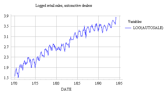
with linear models. For example, here is a graph of
LOG(AUTOSALE). Notice that the log transformation converts
the exponential growth pattern to a linear growth pattern, and
it simultaneously converts the multiplicative (proportional-variance)
seasonal pattern to
an additive (constant-variance) seasonal pattern. (Compare this with
the original
graph of AUTOSALE.)

(Return to top of page.)
Positivity requirement and choice of
base: The logarithm
transformation can be applied only to data which
are strictly positive--you can't take the log of zero or a
negative
number! Also, there are two kinds of logarithms in standard use:
"natural" logarithms and base-10 logarithms. The only
difference between the two is a scaling constant, which is not
really important for modeling purposes. In Statgraphics, the LOG
function is the natural log, and its inverse is the EXP
function. (EXP(Y) is the natural logarithm base, 2.718..., raised
to the Yth power.) The base-10 logarithm and its inverse are LOG10
and EXP10 in Statgraphics. However, in Excel and many hand-held
calculators, the natural logarithm
function is written as LN instead, and LOG stands for the
base-10 logarithm. (Return
to top of page.)
First
difference of LOG = percentage
change: When used in
conjunction with differencing, logging
converts absolute differences into relative (i.e., percentage)
differences. Thus, the series DIFF(LOG(Y)) represents the percentage
change in Y from period to
period. Strictly speaking, the
percentage change in Y at period t is defined as (Y(t)-Y(t-1))/Y(t-1),
which is only approximately equal to LOG(Y(t)) - LOG(Y(t-1)),
but the approximation is almost exact if
the percentage
change is small. In Statgraphics terms, this means that
DIFF(Y)/LAG(Y,1)
is virtually identical to DIFF(LOG(Y)). If you don't believe me,
here's a plot of the percent change in auto sales versus the first
difference of its logarithm, zooming in on the last 5 years. The
blue and red lines are virtually indistinguishable except at the
highest and lowest points.

(Return to top of page.)
The
poor man's deflator: Logging
a series often has an effect very similar to deflating: it dampens
exponential growth patterns and reduces heteroscedasticity
(i.e., stabilizes variance). Logging is therefore a "poor
man's deflator" which does not require any external data (or any
head-scratching about which price index to use). Logging is not exactly
the same as deflating--it
does not eliminate an upward trend in the data--but it
can straighten the trend out so that it can be better fitted by
a linear model. (Compare the logged auto sales graph
with the deflated auto sales graph.)
If you're going to log the data
and then fit a model that implicitly
or explicitly uses differencing (e.g., a random walk,
exponential
smoothing, or ARIMA model), then it is usually redundant to deflate
by a price index, as long as the rate of inflation changes only
slowly: the percentage change measured in nominal dollars will
be nearly the same as the percentange change in constant dollars.
Mathematically speaking, DIFF(LOG(Y/CPI)) is nearly identical
DIFF(LOG(Y)): the only difference between the two is a very faint
amount of noise due to fluctuations in the inflation rate. To
demonstrate this point, here's a graph of the first difference of
logged auto sales, with and without deflation:

By logging rather than
deflating, you avoid the need to incorporate
an explicit forecast of future inflation into the model: you
merely lump inflation together with any other sources of
steady compound growth in the original data. Logging the data before
fitting a random walk model yields a so-called
geometric random walk--i.e., a random walk with geometric
rather than linear growth. A geometric random walk is the default
forecasting model that is commonly used for stock price data. (Return to top of page.)
Trend
in logged units = percentage growth: Because changes in the natural
logarithm are (almost) equal to percentage changes in the original series, it
follows that the slope of a trend line fitted to logged data is equal
to the average percentage growth in the original series.
For example, in the graph of LOG(AUTOSALE) shown
above, if you "eyeball" a trend line you will see that the magnitude of
logged auto sales increases by about 2.5 (from 1.5 to 4.0) over 25
years, which is an average increase of about 0.1 per year, i.e., 10%
per year. It is much easier to estimate this trend from the
logged graph than from the original unlogged one! The 10% figure obtained here is nominal growth,
including inflation. If we had instead eyeballed a trend line on
a plot of
logged deflated sales, i.e.,
LOG(AUTOSALE/CPI), its slope would be the average real
percentage growth.
Usually the
trend is estimated more precisely by fitting a statistical model that
explicitly includes a local or global trend parameter, such as a linear
trend or random-walk-with-drift or linear exponential smoothing
model. When a model of this kind is fitted in conjunction with a
log transformation, its trend parameter can be interpreted as a
percentage growth rate.
Errors in logged
units = percentage
errors: Another interesting
property of the logarithm is
that errors in predicting the logged series can be interpreted
as percentage errors in predicting the original series, albeit
the percentages are relative to the forecast values, not the actual
values. (Normally one interprets the "percentage error"
to be the error expressed as a percentage of the actual value,
not the forecast value, athough the statistical properties of
percentage errors are usually very similar regardless of whether
the percentages are calculated relative to actual values or forecasts.)
Thus, if you use least-squares
estimation to fit a linear forecasting
model to logged data, you are implicitly minimizing mean
squared percentage error, rather than mean squared error
in the original units--which is probably a good thing if the
log transformation was appropriate in the first place. And if
you look at the error statistics in logged units, you can interpret
them as percentages. For example, the standard deviation of the
errors in predicting a logged series is essentially the standard
deviation of the percentage errors in predicting the original
series, and the mean absolute error (MAE) in predicting a logged series
is essentially the mean absolute percentage error (MAPE) in predicting
the original series.
Statgraphics
tip: In the Forecasting procedure in Statgraphics,
the error statistics shown on the Model Comparison report are
all in untransformed (i.e., original) units to facilitate
a comparison among models, regardless of whether they have used
different transformations. (This is a very useful feature of the
Forecasting procedure--in most stat software it is hard to get a
head-to-head comparison of models with and without a log
transformation.) However, whenever a regression model or
an ARIMA model is fitted in conjunction with a log transformation, the
standard-error-of-the-estimate or white-noise-standard-deviation
statistics on the Analysis Summary report refer to the transformed
(logged) errors, in which case they are essentially the RMS percentage errors. (Return to top of page.)


